There is a clever mathematical trick for comparing different data sets, but it does not seem to be widely used. It is based on so-called empirical orthogonal functions (EOFs), which Edward Lorenz described in a Massachusetts Institute of Technology (MIT) scientific report from 1956. The EOFs are similar to principal component analysis (PCA).

The EOFs and PCAs provide patterns of spatio-temporal covariance structure. Usually these techniques are applied to datasets with many parallel variables to show coherent patterns of variability. Myles Allen used to lecture on EOFs at Oxford University about twenty years ago and convinced me about their value. Many scientists do indeed use EOFs to analyse their data.

It is not that there is little use of EOFs (they are widely used), but the question is how the EOFs are used and how the results are interpreted. I learned that EOFs can be used in many different ways from Doug Nychka, when I visited University Corporation for Atmospheric Research (UCAR) in 2011.

The clever trick is to apply these techniques to data compiled from more than one source of data. When used this way, the technique is labelled “common EOFs” or “common PCA”. There are some scientific studies that have made use of common EOFs or common PCA, such as Flurry (1988), Barnett (1999), Sengupta & Boyle (1993), Benestad (2001), and Gilett et al (2002).

Nevertheless, a Scholar Google recent search with “common EOFs” only gave 101 hits (2020-03-05). I find this low interest for this technique a bit puzzling, since it in many ways has lots in common to machine learning and artificial intelligence (AI), both which are hot topics these days.

Common EOFs are also particularly useful for quantifying local effects of global warming through a process known as empirical-statistical downscaling (ESD). It's pity that common EOFs aren't even mentioned in the recent textbook on ESD by Maraun and Widmann (2019)  (they are discussed in Benestad et al. (2008)).
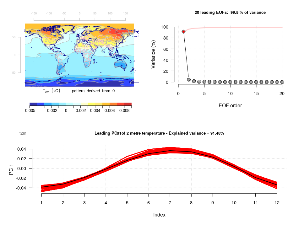
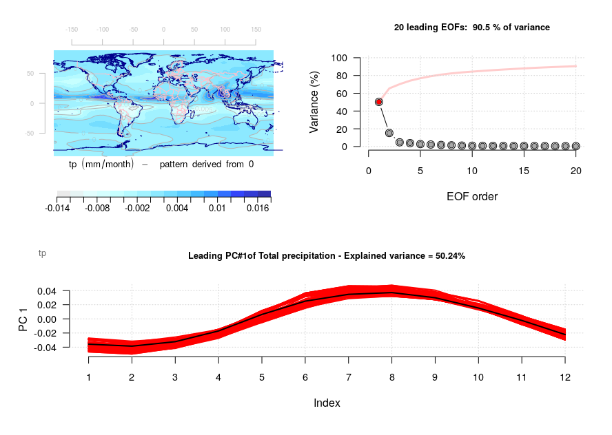
Figure. Examples showing how common EOFs can be used to compare the annual cycle in T(2m) in the upper set of panels and precipitation (lower panels) simulated by global climate models from the CMIP5 experiment (red) and compared with the ERAINT reanalysis (black).
The take-home message from these common EOFs, eigenvalues and principal components, is that the models do reproduce the large-scale patterns in the mean annual cycle. For those interested, common EOFs can easily be calculated with the R-based tool:
github.com/metno/esd.
References
- R.E. Benestad, "A comparison between two empirical downscaling strategies", International Journal of Climatology, vol. 21, pp. 1645-1668, 2001. http://dx.doi.org/10.1002/joc.703
- N.P. Gillett, F.W. Zwiers, A.J. Weaver, G.C. Hegerl, M.R. Allen, and P.A. Stott, "Detecting anthropogenic influence with a multi‐model ensemble", Geophysical Research Letters, vol. 29, 2002. http://dx.doi.org/10.1029/2002GL015836