Some of you that follow my twitter account will have already seen this, but there was a particularly amusing episode of Q&A on Australian TV that pitted Prof. Brian Cox against a newly-elected politician who is known for his somewhat fringe climate ‘contrarian’ views. The resulting exchanges were fun:
[Read more…] about Australian silliness and July temperature records
Climate Science
Unforced variations: Aug 2016
Sorry for the low rate of posts this summer. Lots of offline life going on. ;-)
Meantime, this paper by Hourdin et al on climate model tuning is very interesting and harks back to the FAQ we did on climate models a few years ago (Part I, Part II). Maybe it’s worth doing an update?
Some of you might also have seen some of the discussion of record temperatures in the first half of 2016. The model-observation comparison including the estimates for 2016 are below:
It seems like the hiatus hiatus will continue…
Unforced variations: July 2016
A week is a long time in politics climate science: Nonsense debunked in WaPo, begininngs of recovery in the ozone hole, revisiting the instrumental record constraints on climate sensitivity…
Lots of lessons there.
Usual rules apply.
Boomerangs versus Javelins: The Impact of Polarization on Climate Change Communication
Guest commentary by Jack Zhou, Nicholas School of the Environment, Duke University
For advocates of climate change action, communication on the issue has often meant “finding the right message” that will spur their audience to action and convince skeptics to change their minds. This is the notion that simply connecting climate change to the right issue domains or symbols will cut through the political gridlock on the issue. The difficulty then lies with finding these magic bullet messages, figuring out if they talk about climate change in the context of with national security or polar bears or passing down a clean environment to future generations.
On highly polarized issues like climate change, however, communicating across the aisle may be more difficult than simply finding the right message. Here, the worst case scenario is not simply a message failing to land and sending you back to the drawing board. Instead, any message that your audience disagrees with may polarize that audience even further in their skepticism, leaving you in a worse position than you began. As climate change has become an increasingly partisan issue in American politics, this means that convincing Republicans to reject the party line of climate skepticism may be easier said than done.
[Read more…] about Boomerangs versus Javelins: The Impact of Polarization on Climate Change Communication
Unforced Variations: June 2016
Do regional climate models add value compared to global models?
Global climate models (GCM) are designed to simulate earth’s climate over the entire planet, but they have a limitation when it comes to describing local details due to heavy computational demands. There is a nice TED talk by Gavin that explains how climate models work.
We need to apply downscaling to compute the local details. Downscaling may be done through empirical-statistical downscaling (ESD) or regional climate models (RCMs) with a much finer grid. Both take the crude (low-resolution) solution provided by the GCMs and include finer topographical details (boundary conditions) to calculate more detailed information. However, does more details translate to a better representation of the world?
The question of “added value” was an important topic at the International Conference on Regional Climate conference hosted by CORDEX of the World Climate Research Programme (WCRP). The take-home message was mixed on whether RCMs provide a better description of local climatic conditions than the coarser GCMs.
[Read more…] about Do regional climate models add value compared to global models?
AMOC slowdown: Connecting the dots
I want to revisit a fascinating study that recently came from (mainly) the Geophysical Fluid Dynamics Lab in Princeton. It looks at the response of the Atlantic Ocean circulation to global warming, in the highest model resolution that I have seen so far. That is in the CM2.6 coupled climate model, with 0.1° x 0.1° degrees ocean resolution, roughly 10km x 10km. Here is a really cool animation.
When this model is run with a standard, idealised global warming scenario you get the following result for global sea surface temperature changes.
Fig. 1. Sea surface temperature change after doubling of atmospheric CO2 concentration in a scenario where CO2 increases by 1% every year. From Saba et al. 2016.
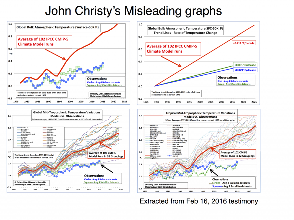
Comparing models to the satellite datasets
How should one make graphics that appropriately compare models and observations? There are basically two key points (explored in more depth here) – comparisons should be ‘like with like’, and different sources of uncertainty should be clear, whether uncertainties are related to ‘weather’ and/or structural uncertainty in either the observations or the models. There are unfortunately many graphics going around that fail to do this properly, and some prominent ones are associated with satellite temperatures made by John Christy. This post explains exactly why these graphs are misleading and how more honest presentations of the comparison allow for more informed discussions of why and how these records are changing and differ from models.
[Read more…] about Comparing models to the satellite datasets
Unforced variations: May 2016
Nenana Ice Classic 2016
Just a quick note since I’ve been tracking this statistic for a few years, but the Nenana Ice Classic tripod went down this afternoon (Apr 23, 3:39 Alaska Standard Time). See the earlier post for what this is and why it says something about the climate (see posts on 2014 and 2015 results).
With this unofficial time, this year places 4th earliest for the breakup of ice in the Tanana river. It is unsurprising that it was early given the exceptional warmth in Alaska this year.
The exact ranking of years depends a little on how one accounts for leap-year and other calendrical effects. The raw date is the 4th earliest, but given that this year is a leap year, it would be the 5th earliest counting Julian days from the start of the year. Tying the season to the vernal equinox is more stable, which again leads to the 4th earliest. But regardless of that detail, and consistent with local climate warming, the ice break-up date have advanced about 7 days over the last century.
As a side bet, I predict (based on previous years) that despite enormous attention in the skeptic-osphere given the Nenana result in 2013 (when it was remarkably late), it won’t be mentioned there this year.