• Skip to primary navigation
  • Skip to main content
  • Skip to primary sidebar
  • Skip to footer

RealClimate

Climate science from climate scientists...

  • Start here
  • Model-Observation Comparisons
  • Miscellaneous Climate Graphics
  • Surface temperature graphics
You are here: Home / Archives for Gavin

about Gavin Schmidt

Gavin Schmidt is a climate modeler, working for NASA and with Columbia University.

Younger Dry-as dust?

24 Oct 2007 by Gavin

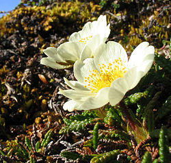
The Younger Dryas is so called because it corresponds, in the pollen record from Europe, to the latest (i.e. youngest) appearance of the Dryas octopetala pollen, an alpine flower in regions that are now far from alpine. It marks a clear period towards the end of the last ice age when the warming trend of the deglaciation in Europe particularly was interrupted for a period of about 1300 years before it got going again. There were clear glacier advances during this time and the moraines can be seen very clearly all around Europe and Scandinavia.

The clues to what caused this remarkable, if temporary, turnaround have always lain in assessing its spatial extent, the exact timing and correspondence with other events. Two recent papers have shed some welcome and potentially controversial light on the subject.

[Read more…] about Younger Dry-as dust?

Filed Under: Climate Science, Oceans, Paleoclimate

CO2 equivalents

11 Oct 2007 by Gavin

There was a minor kerfuffle in recent days over claims by Tim Flannery (author of “The Weather Makers”) that new information from the upcoming IPCC synthesis report will show that we have reached 455 ppmv CO2_equivalent 10 years ahead of schedule, with predictable implications. This is confused and incorrect, but the definitions of CO2_e, why one would use it and what the relevant level is, are all highly uncertain in many peoples’ minds. So here is a quick rundown.

Definition: The CO2_equivalent level is the amount of CO2 that would be required to give the same global mean radiative forcing as the sum of a basket of other forcings. This is a way to include the effects of CH4 and N2O etc. in a simple way, particularly for people doing future impacts or cost-benefit analysis. The equivalent amount is calculated using the IPCC formula for CO2 forcing:

Total Forcing = 5.35 log(CO2_e/CO2_orig)

where CO2_orig is the 1750 concentration (278 ppmv).

Usage: There are two main ways it is used. Firstly, it is often used to group together all the forcings from the Kyoto greenhouse gases (CO2, CH4, N2O and CFCs), and secondly to group together all forcings (including ozone, sulphate aerosols, black carbon etc.). The first is simply a convenience, but the second is what matters to the planet. Many stabilisation scenarios, such as are being discussed in UNFCCC negotiations are based on stabilising total CO2_e at 450, 550 or 750 ppmv.

Magnitude The values of CO2_e (Kyoto) and CO2_e (Total) can be calculated from Figure 2.21 and Table 2.12 in the IPCC WG1 Chapter 2. The forcing for CO2, CH4 (including indirect effects), N2O and CFCs is 1.66+0.48+0.07+0.16+0.34=2.71 W/m2 (with around 0.3 W/m2 uncertainty). Using the formula above, that gives CO2_e (Kyoto) = 460 ppmv. However, including all the forcings (some of which are negative), you get a net forcing of around 1.6 W/m2, and a CO2_e (Total) of 375 ppmv with quite a wide error bar. This is, coincidently, close to the actual CO2 level.

Implications The important number is CO2_e (Total) which is around 375 ppmv. Stabilisation scenarios of 450 ppmv or 550 ppmv are therefore still within reach. Claims that we have passed the first target are simply incorrect, however, that is not to say they are easily achievable. It is even more of a stretch to state that we have all of a sudden gone past the ‘dangerous’ level. It is still not clear what that level is, but if you take a conventional 450 ppmv CO2_e value (which will lead to a net equilibrium warming of ~ 2 deg C above pre-industrial levels), we are still a number of years from that, and we have (probably) not yet committed ourselves to reaching it.

Finally, the IPCC synthesis report is simply a concise summary of the three separate reports that have already come out. It therefore can’t be significantly different from what is already available. But this is another example where people are quoting from draft reports that they have neither properly read nor understood and for which better informed opinion is not immediately available. I wish journalists and editors would resist the temptation to jump on leaks like this (though I know it’s hard). The situation is confusing enough without adding to it unintentionally.

Filed Under: Climate Science, Greenhouse gases, IPCC

Perspectives from China

26 Sep 2007 by Gavin

I spent the last three weeks in China partly for a conference, partly for a vacation, and partly for a rest. In catching up over the last couple of days, I notice that the break has given me a slightly different perspective on a couple of issues that are relevant here.

First off, the conference I attended was on paleoceanography and there were was a lot of great new science presented, particularly concerning the Paleocene-Eocene Thermal Maximum (around 55 million years ago), and on past changes to tropical rainfall patterns (see this week’s Nature) – two issues where there is a lot of relevance for climate change and its impacts today. I’ll discuss the new data in separate posts over the next few weeks, but for now I’ll just mention a topic that came up repeatedly in conversations over the week – that was how to improve the flow of information from the paleo community to the wider climate community, as represented by the IPCC for instance.

There was a palpable sense that insights from paleo-climate (in this case referring mainly to the ocean sediment record rather than ice cores or records from the last millennium) were not being given their due, and in fact were frequently being misused. In a panel discussion (hosted by Stefan), people lamented the lack of ‘synthesis’ that would be useful for the outside community, while others stressed (correctly) that synthesis is hard and frankly not well regarded within the community or their funders. I think this is a general problem; many of the incentives for success within an academic field – the push for novel techniques, the ownership of specific slices of data, the desire to emulate the paths to success of the previous generation – actually discourage work across the field that pulls together disparate sources of information.

In the paleo-oceanography case, this exhibits itself in the overwhelming focus on downcore records (the patterns of change at a single point through time) and the relative lack of integrated products that either show spatial patterns of change at a single time, or that try to extract common elements from multiple events in the past. There are of course numerous exceptions – the MARGO project that compiled records from the peak of the last ice age, or the work of PMIP for the mid-Holocene – but their visibility makes their uniqueness all the more obvious. There were no ideas presented that would fix this overnight, but the discussions showed that the community realises that there is a problem – even if the solutions are elusive.

My second thought on China came from travelling through some of the most polluted cites in the world. Aerosol haze that appeared continuous from Beijing to Hong Kong is such an obvious sign of human industrial activity that it simply takes your breath away (literally). In places, even on a clear day, you cannot see the sun – even if there is no cloud in the sky. Only in the mountains or in deeply rural parts of the country was blue sky in evidence. This is clearly an unsustainable situation (even if you are only thinking about the human health impacts) and it points the way, I think, to how China can be engaged on the climate change front. If reducing aerosol emissions can be done at the same time that greenhouse gases can be cut, the Chinese will likely jump at the chance. As an aside, I noticed that Compact Florescent Light bulbs were being used almost everywhere you looked, and that the majority of Shanghai’s motorbikes and scooters were electric rather than gasoline powered. These efforts clearly help, but they are just as clearly not sufficient on their own.

Finally, the limited access to the Internet that one gets in China (through a combination of having better things to do with one’s time and the sometimes capricious nature of what gets through the Great Firewall) allowed me to take a bit of break from the constant back and forth on the climate blogs. In getting back into it, one appreciates just how much time is wasted dealing with the most ridiculous of issues (Hansen’s imagined endorsement of a paper he didn’t write thirty six years ago, the debunking of papers that even E&E won’t publish, and the non-impact of the current fad for amateur photography) at the expense of anything substantive. In effect, if possibly not in intention, this wastes a huge amount of people’s time and diverts attention from more significant issues (at least in the various sections of the blogosphere). Serious climate bloggers might all benefit from not getting too caught up in it, and keeping an closer eye on the bigger picture. We will continue to try and do so here.

Filed Under: Aerosols, Climate Science, Paleoclimate

Who ya gonna call?

22 Aug 2007 by Gavin

Gavin Schmidt and Michael Mann

Scientific theories gain credence from successful predictions. Similarly, scientific commentators should gain credibility from whether their comments on new studies hold up over time. Back in 2005 we commented on the Bryden et al study on a possible ongoing slowdown in the North Atlantic overturning circulation. In our standard, scientifically cautious, way we said:

… it might be premature to assert that the circulation definitely has changed.

Our conclusion that the Bryden et al result ‘might be premature’ was based on a balance of evidence argument (or, since we discussed this a few days ago, our Bayesian priors) for what the consequences of such a slowdown would be (a (unobserved) cooling in the North Atlantic). We also reported last year on some data that would likely help assess the uncertainty.

Well, now that data has been properly published (reported here) and it confirms what we thought all along. The sampling variability in the kind of snapshot surveys that Bryden et al had used was too large for the apparent trends that they saw to be significant (which the authors had correctly anticipated in the original paper though).

Score one for Bayesian priors.

Filed Under: Climate Science, Oceans

Musings about models

20 Aug 2007 by Gavin

With the blogosphere all a-flutter with discussions of hundredths of degrees adjustments to the surface temperature record, you probably missed a couple of actually interesting stories last week.

Tipping points

Oft-discussed and frequently abused, tipping points are very rarely actually defined. Tim Lenton does a good job in this recent article. A tipping ‘element’ for climate purposes is defined as

The parameters controlling the system can be transparently combined into a single control, and there exists a critical value of this control from which a small perturbation leads to a qualitative change in a crucial feature of the system, after some observation time.

and the examples that he thinks have the potential to be large scale tipping elements are: Arctic sea-ice, a reorganisation of the Atlantic thermohaline circulation, melt of the Greenland or West Antarctic Ice Sheets, dieback of the Amazon rainforest, a greening of the Sahara, Indian summer monsoon collapse, boreal forest dieback and ocean methane hydrates.

To that list, we’d probably add any number of ecosystems where small changes can have cascading effects – such as fisheries. It’s interesting to note that most of these elements include physics that modellers are least confident about – hydrology, ice sheets and vegetation dynamics.

Prediction vs. Projections

As we discussed recently in connection with climate ‘forecasting‘, the kinds of simulations used in AR4 are all ‘projections’ i.e. runs that attempt to estimate the forced response of the climate to emission changes, but that don’t attempt to estimate the trajectory of the unforced ‘weather’. As we mentioned briefly, that leads to a ‘sweet spot’ for forecasting of a couple of decades into the future where the initial condition uncertainty dies away, but the uncertainty in the emission scenario is not yet so large as to be dominating. Last week there was a paper by Smith and colleagues in Science that tried to fill in those early years, using a model that initialises the heat content from the upper ocean – with the idea that the structure of those anomalies control the ‘weather’ progression over the next few years.

They find that their initialisation makes a difference for a about a decade, but that at longer timescales the results look like the standard projections (i.e. 0.2 to 0.3ºC per decade warming). One big caveat is that they aren’t able to predict El Niño events, and since they account for a great deal of the interannual global temperature anomaly, that is a limitation. Nonetheless, this is a good step forward and people should be looking out for whether their predictions – for a plateau until 2009 and then a big ramp up – materialise over the next few years.

Model ensembles as probabilities

A rather esoteric point of discussion concerning ‘Bayesian priors’ got a mainstream outing this week in the Economist. The very narrow point in question is to what extent model ensembles are probability distributions. i.e. if only 10% of models show a particular behaviour, does this mean that the likelihood of this happening is 10%?

The answer is no. The other 90% could all be missing some key piece of physics.

However, there has been a bit of confusion generated though through the work of climateprediction.net – the multi-thousand member perturbed parameter ensembles that, notoriously, suggested that climate sensitivity could be as high as 11 ºC in a paper a couple of years back. The very specific issue is whether the histograms generated through that process could be considered a probability distribution function or not. (‘Not’ is the correct answer).

The point in the Economist article is that one can demonstrate that very clearly by changing the variables you are perturbing (in the example they use an inverse). If you evenly sample X, or evenly sample 1/X (or any other function of X) you will get a different distribution of results. Then instead of (in one case) getting 10% of models runs to show behaviour X, now maybe 30% of models will. And all this is completely independent of any change to the physics.

My only complaint about the Economist piece is the conclusion that, because of this inherent ambiguity, dealing with it becomes a ‘logistical nightmare’ – that’s is incorrect. What should happen is that people should stop trying to think that counting finite samples of model ensembles can give a probability. Nothing else changes.

Filed Under: Climate modelling, Climate Science

1934 and all that

10 Aug 2007 by Gavin

Another week, another ado over nothing.

Last Saturday, Steve McIntyre wrote an email to NASA GISS pointing out that for some North American stations in the GISTEMP analysis, there was an odd jump in going from 1999 to 2000. On Monday, the people who work on the temperature analysis (not me), looked into it and found that this coincided with the switch between two sources of US temperature data. There had been a faulty assumption that these two sources matched, but that turned out not to be the case. There were in fact a number of small offsets (of both sign) between the same stations in the two different data sets. The obvious fix was to make an adjustment based on a period of overlap so that these offsets disappear.

This was duly done by Tuesday, an email thanking McIntyre was sent and the data analysis (which had been due in any case for the processing of the July numbers) was updated accordingly along with an acknowledgment to McIntyre and update of the methodology.

The net effect of the change was to reduce mean US anomalies by about 0.15 ºC for the years 2000-2006. There were some very minor knock on effects in earlier years due to the GISTEMP adjustments for rural vs. urban trends. In the global or hemispheric mean, the differences were imperceptible (since the US is only a small fraction of the global area).

There were however some very minor re-arrangements in the various rankings (see data [As it existed in Sep 2007]). Specifically, where 1998 (1.24 ºC anomaly compared to 1951-1980) had previously just beaten out 1934 (1.23 ºC) for the top US year, it now just misses: 1934 1.25ºC vs. 1998 1.23ºC. None of these differences are statistically significant. Indeed in the 2001 paper describing the GISTEMP methodology (which was prior to this particular error being introduced), it says:

The U.S. annual (January-December) mean temperature is slightly warmer in 1934 than in 1998 in the GISS analysis (Plate 6). This contrasts with the USHCN data, which has 1998 as the warmest year in the century. In both cases the difference between 1934 and 1998 mean temperatures is a few hundredths of a degree. The main reason that 1998 is relatively cooler in the GISS analysis is its larger adjustment for urban warming. In comparing temperatures of years separated by 60 or 70 years the uncertainties in various adjustments (urban warming, station history adjustments, etc.) lead to an uncertainty of at least 0.1°C. Thus it is not possible to declare a record U.S. temperature with confidence until a result is obtained that exceeds the temperature of 1934 by more than 0.1°C.

More importantly for climate purposes, the longer term US averages have not changed rank. 2002-2006 (at 0.66 ºC) is still warmer than 1930-1934 (0.63 ºC – the largest value in the early part of the century) (though both are below 1998-2002 at 0.79 ºC). (The previous version – up to 2005 – can be seen here).

In the global mean, 2005 remains the warmest (as in the NCDC analysis). CRU has 1998 as the warmest year but there are differences in methodology, particularly concerning the Arctic (extrapolated in GISTEMP, not included in CRU) which is a big part of recent global warmth. No recent IPCC statements or conclusions are affected in the slightest.

Sum total of this change? A couple of hundredths of degrees in the US rankings and no change in anything that could be considered climatically important (specifically long term trends).

However, there is clearly a latent and deeply felt wish in some sectors for the whole problem of global warming to be reduced to a statistical quirk or a mistake. This led to some truly death-defying leaping to conclusions when this issue hit the blogosphere. One of the worst examples (but there are others) was the ‘Opinionator’ at the New York Times (oh dear). He managed to confuse the global means with the continental US numbers, he made up a story about McIntyre having ‘always puzzled about some gaps’ (what?) , declared the the error had ‘played havoc’ with the numbers, and quoted another blogger saying that the ‘astounding’ numbers had been ‘silently released’. None of these statements are true. Among other incorrect stories going around are that the mistake was due to a Y2K bug or that this had something to do with photographing weather stations. Again, simply false.

But hey, maybe the Arctic will get the memo.

Filed Under: Climate Science, Instrumental Record

The CO2 problem in 6 easy steps

6 Aug 2007 by Gavin

We often get requests to provide an easy-to-understand explanation for why increasing CO2 is a significant problem without relying on climate models and we are generally happy to oblige. The explanation has a number of separate steps which tend to sometimes get confused and so we will try to break it down carefully.
[Read more…] about The CO2 problem in 6 easy steps

Filed Under: Climate Science, Greenhouse gases

Ozone impacts on climate change

27 Jul 2007 by Gavin

In a nice example of how complicated climate feedbacks and interactions can be, Sitch and colleagues report in Nature advance publication on a newly modelled effect of ground level (or tropospheric) ozone on carbon uptake on land (BBC). The ozone they are talking about is the ‘bad’ ozone (compared to ‘good’ stratospheric ozone) and is both a public health hazard and a greenhouse gas. Tropospheric ozone isn’t directly emitted by human activity, but is formed in the atmosphere as a result of photolytic reactions related to CH4, CO, NOx and VOCs (Volatile Organic Compounds like isoprene, benzene etc.) – the so-called ozone precursors.

It’s well known that increased ozone levels – particularly downwind of cities – can be harmful to plants, and in this new study with a carbon-climate model, they quantify how by how much increasing ozone levels make it more difficult for carbon to be sequestered by the land biosphere. This leads to larger CO2 levels in the atmosphere than before. Hence the ozone has, as well as its direct effect as a greenhouse gas, an indirect effect on CO2, which in this model at least appears to be almost as large.

Actually it’s even more complicated. Methane emissions are one of the principal causes of the rise of ozone, and the greenhouse effect of ozone can be thought of as an indirect effect of CH4 (and CO and VOCs). But while NOx is an ozone precursor, it actually has an indirect effect that reduces CH4, so that the net impact of NOx has been thought to be negative (i.e. the reduction in CH4 outweighs the increase of ozone in radiative forcing – see this paper for more details). This new result might prompt a re-adjustment of that balance – i.e. if the ozone produced by NOx has a stronger effect than previously thought (through this new indirect mechanism), than it might outweigh the reduction in CH4, and lead to NOx emissions themselves being a (slightly) positive forcing.

In a bizarre way this is actually good news. There are plenty of reasons to reduce NOx emissions already because of it’s impact on air pollution and smog, but this new result might mean that reductions wouldn’t make climate change any worse. It also, once again, highlights the role of CH4 (the second biggest GHG forcing), and points out a further reason (if that was required) why further methane reductions could be particularly welcome in moderating future changes in climate and air quality.

Filed Under: Climate Science, Greenhouse gases

Green and Armstrong’s scientific forecast

20 Jul 2007 by Gavin

There is a new critique of IPCC climate projections doing the rounds of the blogosphere from two ‘scientific forecasters’, Kesten Green and Scott Armstrong, who claim that since the IPCC projections are not ‘scientific forecasts’ they must perforce be wrong and that a naive model of no change in future is likely to be more accurate that any IPCC conclusion. This ignores the fact that IPCC projections have already proved themselves better than such a naive model, but their critique is novel enough to be worth a mention.
[Read more…] about Green and Armstrong’s scientific forecast

Filed Under: Climate modelling, Climate Science, IPCC

Making sense of Greenland’s ice

9 Jul 2007 by Gavin

A widely publicised paper in Science last week discussed the recovery ancient DNA from the base of the Dye-3 ice core (in southern Greenland). This was an impressive technical feat and the DNA recovered may well be the oldest pure DNA ever, dating back maybe half a million years. However much of the press coverage of this paper dwelt not on the positive aspects of the study but on its supposed implications for the stability of the Greenland ice sheet and future sea level rise, something that was not greatly discussed in the paper at all. So why was this?
[Read more…] about Making sense of Greenland’s ice

Filed Under: Arctic and Antarctic, Climate Science, Paleoclimate

  • « Go to Previous Page
  • Page 1
  • Interim pages omitted …
  • Page 28
  • Page 29
  • Page 30
  • Page 31
  • Page 32
  • Interim pages omitted …
  • Page 40
  • Go to Next Page »

Primary Sidebar

Search

Search for:

Email Notification

get new posts sent to you automatically (free)
Loading

Recent Posts

  • Unforced variations: May 2025
  • Unforced Variations: Apr 2025
  • WMO: Update on 2023/4 Anomalies
  • Andean glaciers have shrunk more than ever before in the entire Holocene
  • Climate change in Africa
  • We need NOAA now more than ever

Our Books

Book covers
This list of books since 2005 (in reverse chronological order) that we have been involved in, accompanied by the publisher’s official description, and some comments of independent reviewers of the work.
All Books >>

Recent Comments

  • Tomáš Kalisz on Unforced variations: May 2025
  • Secular Animist on Unforced variations: May 2025
  • Secular Animist on Unforced variations: May 2025
  • Barry E Finch on Unforced variations: May 2025
  • Radge Havers on Unforced variations: May 2025
  • Barton Paul Levenson on Unforced variations: May 2025
  • jgnfld on Unforced variations: May 2025
  • jgnfld on Unforced variations: May 2025
  • zebra on Unforced variations: May 2025
  • Thessalonia on Unforced variations: May 2025
  • Mr. Know It All on Unforced variations: May 2025
  • Mr. Know It All on Unforced variations: May 2025
  • Mr. Know It All on Unforced variations: May 2025
  • Pedro Prieto on Unforced variations: May 2025
  • Pedro Prieto on Unforced variations: May 2025
  • Nigelj on Unforced variations: May 2025
  • Piotr on Unforced variations: May 2025
  • Piotr on Unforced variations: May 2025
  • Killian on Unforced variations: May 2025
  • Killian on Unforced variations: May 2025

Footer

ABOUT

  • About
  • Translations
  • Privacy Policy
  • Contact Page
  • Login

DATA AND GRAPHICS

  • Data Sources
  • Model-Observation Comparisons
  • Surface temperature graphics
  • Miscellaneous Climate Graphics

INDEX

  • Acronym index
  • Index
  • Archives
  • Contributors

Realclimate Stats

1,364 posts

11 pages

242,910 comments

Copyright © 2025 · RealClimate is a commentary site on climate science by working climate scientists for the interested public and journalists.