Unforced Variations vs Forced Responses?

Guest commentary by Karsten Haustein, U. Oxford, and Peter Jacobs (George Mason University).

One of the perennial issues in climate research is how big a role internal climate variability plays on decadal to longer timescales. A large role would increase the uncertainty on the attribution of recent trends to human causes, while a small role would tighten that attribution. There have been a number of attempts to quantify this over the years, and we have just published a new study (Haustein et al, 2019) in the Journal of Climate addressing this question.

Using a simplified climate model, we find that we can reproduce temperature observations since 1850 and proxy-data since 1500 with high accuracy. Our results suggest that multidecadal ocean oscillations are only a minor contributing factor in the global mean surface temperature evolution (GMST) over that time. The basic results were covered in excellent articles in CarbonBrief and Science Magazine, but this post will try and go a little deeper into what we found.

Until recently, the hypothesis that there are significant natural (unforced) ocean cycles with an approximate periodicity of 60-70 years had been widely accepted. The so-called Atlantic Multidecadal Variability index (AMV, sometimes called the AMO instead), but also the Pacific Decadal Variability index (PDV) have been touted as major factors in observed multidecadal GMST fluctuations (for instance, here). Due to the strong co-variability between AMV and GMST, both, the Early 20^th Century Warming (1915-1945) and the Mid-Century Cooling (1950-1980) have been attributed to low-frequency AMV variability, associated to a varying degree with changes in the Atlantic Meridional Overturning Circulation (AMOC). In particular, the uncertainty in quantifying the human-induced warming fraction in the early 20th Century was still substantial.

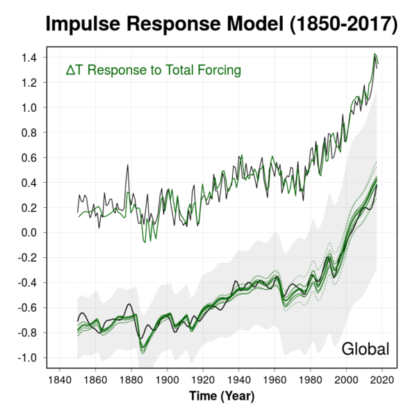
In contrast to those earlier studies, we were able to reproduce effectively all the observed multidecadal temperature evolution, including the Early Warming and the Mid-Century cooling, using known external forcing factors (solar activity, volcanic eruptions, greenhouse gases, pollution aerosol particles). Adding an El Niño signal, we virtually explain the entire observed record (Figure 1). Further, we were able to reproduce the temperature evolution separately over land and ocean, and between Northern and Southern Hemispheres (NH/SH). We found equally high fractions of explained variability associated with anthropogenic and natural radiative forcing changes in each case. Attributing 90% of the Early Warming to external forcings (50% of which is due to natural forcing from volcanoes and solar) is – in our view – a key leap forward. To date, no more than 50% had been attributed to external forcing (Hegerl et al. 2018). While there is less controversy about the drivers of the Mid-Century cooling, our response model results strongly support the idea that the trend was caused by increased levels of sulphate aerosols which temporarily offset greenhouse gas-induced warming.

What does this mean?

Some commentators have used the uncertainty in the attribution for the Early 20th Century warming as an excuse to not accept the far stronger evidence for the human causes of more recent trends (notably, Judith Curry). This was never very convincing, but is even further diminished given a viable attribution for the Early Warming now exists. Despite a number of studies that have already provided evidence – based on a solid physical underpinning – for a large external contribution to observed multidecadal ocean variability, most prominently the AMV (e.g. Mann et al., 2014; Clement et al., 2015, Stolpe et al. 2017), ideas such as the stadium wave (Wyatt and Curry, 2014) continue to be proposed. The problem is that most studies that argue for unforced low-frequency ocean oscillations do not accommodate time-varying external drivers such as anthropogenic aerosols. Our findings highlight that this non-linearity is a crucial feature of the historic forcing evolution. Any claim that these forcings were/are small has to be accompanied by solid evidence disproving the observed multidecadal variations in incoming radiation (e.g. Wild 2009). On the contrary, our findings confirm that the fraction of human-induced warming since the pre-industrial era is bascially all of it.

Implications

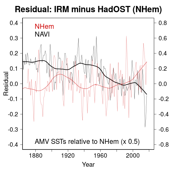
We conclude that the AMV time series (based on the widely accepted definition) almost certainly does not represent a simple internal mode of variability. Indeed, we think that the AMV definition is flawed and not a suitable method to extract whatever internal ocean signal there might be. Instead we recommend the use of an alternative index which we think will be closer to the internal signal, called the North Atlantic Variability Index (NAVI). It is essentially the AMV relative to the NH temperature (Figure 2). The resulting timeseries of the new NAVI index is a good representation of the AMOC decline, arguably the true internal component (although also forcing-related) in the North Atlantic. This implies that while the AMOC is an important player (see for instance, Stefan’s RC post), it is not driving alleged low-frequency North Atlantic ocean oscillations. The AMV should therefore not be used as predictor in attribution studies given that the multidecadal temperature swings are unlikely internally generated. Though we note that the projection of AMV on GMST is small in any case.

What did our results rely on?

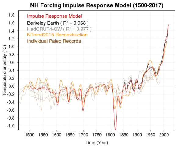
There are three novelties that led to our conclusions: (1) We differentiate between forcing factors such as volcanoes and pollution aerosols with regard to their transient climate response (TCR). For example, anthropogenic aerosols are primarily emitted over NH continents, i.e. they have a faster TCR which we explicitly account for in our analysis. (2) We use an updated aerosol emission dataset (CEDS, Hoesly et al., 2017, also used in CMIP6), resulting in a substantially different temporal evolution of historic aerosol emissions compared to the older dataset (Lamarque et al. 2010). The effective aerosol forcing is based on the most recent estimate by [9]. (3) The final change is related to the observational data. The HadISST1/2 (Kennedy et al. in prep) ocean temperature dataset (SST) has never been used in conjunction with land data. We have combined HadISST2 with Cowtan/Way over land (using air temperature over sea ice) and filled the missing years after 2010 with OSTIA SSTs (due to it being preliminary only). In addition, it has been known for quite some time now that there is a bias in virtually all  SST dataset during the 2^nd world war (Cowtan et al., 2018, and see also Kevin’s SkS post). We correct for that bias over ocean (1942-1945), which, in conjunction with warmer HadISST2 SSTs before the 1930s, significantly reduced previous discrepancies related to the Early Warming. Lastly, the fact that the model is initialised in 1500 A.D. ensures that the slow response to strong volcanic eruptions is sensibly accounted for (Figure 3), as it has shown to be important on centennial timescales (e.g. Gleckler et al. 2006).

What about overfitting?

In order to address this issue, we would like to point out that not a single parameter depends on regression. TCR and ECS span a wide range of accepted values and all we did is to estimate TCR based on the best fit of the final response model result with observations. We concede that the fast response time and the effective aerosol forcing are difficult to pin down given there is a wide range of published estimates available. However, it is worth mentioning that the results are not very sensitive to variations in both parameters (see thin lines in Figure 1). Instead, the overall uncertainty is dominated by the TCR and GHG forcing uncertainty. The story is more complex when it comes to the NH/SH and land/ocean-only results as we need to account for the different warming-ratios. Guided by climate model and observational data, we introduce a novel method that objectively estimates the required TCR factors.

Conclusions: It was us.

The findings presented in our paper highlight that we are now able to explain almost all the warming patterns since 1850, including the Early Warming period. We achieve this by separating different forcing factors, by including an updated aerosol dataset and by removing notable SST biases. We have avoided overfitting by virtue of a strict non-regression policy. We ask the different research communities to take these findings as food for thought, particularly with regard to the Early Warming. We most definitely believe that it is time to rethink the role of the AMV and recommend using our newly introduced NAVI definition instead. This will also help to understand contemporary AMOC changes and its relation to climate change better, and perhaps provide guidance as to which climate models best approximate internal ocean variability on longer timescales.

References

1. K. Haustein, F.E.L. Otto, V. Venema, P. Jacobs, K. Cowtan, Z. Hausfather, R.G. Way, B. White, A. Subramanian, and A.P. Schurer, "A Limited Role for Unforced Internal Variability in Twentieth-Century Warming", Journal of Climate, vol. 32, pp. 4893-4917, 2019. http://dx.doi.org/10.1175/JCLI-D-18-0555.1
2. G.C. Hegerl, S. Brönnimann, A. Schurer, and T. Cowan, "The early 20th century warming: Anomalies, causes, and consequences", WIREs Climate Change, vol. 9, 2018. http://dx.doi.org/10.1002/wcc.522
3. M.E. Mann, B.A. Steinman, and S.K. Miller, "On forced temperature changes, internal variability, and the AMO", Geophysical Research Letters, vol. 41, pp. 3211-3219, 2014. http://dx.doi.org/10.1002/2014GL059233
4. A. Clement, K. Bellomo, L.N. Murphy, M.A. Cane, T. Mauritsen, G. Rädel, and B. Stevens, "The Atlantic Multidecadal Oscillation without a role for ocean circulation", Science, vol. 350, pp. 320-324, 2015. http://dx.doi.org/10.1126/science.aab3980
5. M.B. Stolpe, I. Medhaug, and R. Knutti, "Contribution of Atlantic and Pacific Multidecadal Variability to Twentieth-Century Temperature Changes", Journal of Climate, vol. 30, pp. 6279-6295, 2017. http://dx.doi.org/10.1175/JCLI-D-16-0803.1
6. M.G. Wyatt, and J.A. Curry, "Role for Eurasian Arctic shelf sea ice in a secularly varying hemispheric climate signal during the 20th century", Climate Dynamics, vol. 42, pp. 2763-2782, 2013. http://dx.doi.org/10.1007/s00382-013-1950-2
7. M. Wild, "Global dimming and brightening: A review", Journal of Geophysical Research: Atmospheres, vol. 114, 2009. http://dx.doi.org/10.1029/2008JD011470
8. R.M. Hoesly, S.J. Smith, L. Feng, Z. Klimont, G. Janssens-Maenhout, T. Pitkanen, J.J. Seibert, L. Vu, R.J. Andres, R.M. Bolt, T.C. Bond, L. Dawidowski, N. Kholod, J. Kurokawa, M. Li, L. Liu, Z. Lu, M.C.P. Moura, P.R. O'Rourke, and Q. Zhang, "Historical (1750–2014) anthropogenic emissions of reactive gases and aerosols from the Community Emissions Data System (CEDS)", Geoscientific Model Development, vol. 11, pp. 369-408, 2018. http://dx.doi.org/10.5194/gmd-11-369-2018
9. C.E. Forest, "Inferred Net Aerosol Forcing Based on Historical Climate Changes: a Review", Current Climate Change Reports, vol. 4, pp. 11-22, 2018. http://dx.doi.org/10.1007/s40641-018-0085-2
10. K. Cowtan, R. Rohde, and Z. Hausfather, "Evaluating biases in sea surface temperature records using coastal weather stations", Quarterly Journal of the Royal Meteorological Society, vol. 144, pp. 670-681, 2018. http://dx.doi.org/10.1002/qj.3235
11. P.J. Gleckler, K. AchutaRao, J.M. Gregory, B.D. Santer, K.E. Taylor, and T.M.L. Wigley, "Krakatoa lives: The effect of volcanic eruptions on ocean heat content and thermal expansion", Geophysical Research Letters, vol. 33, 2006. http://dx.doi.org/10.1029/2006GL026771