In an earlier post, we discussed a review article by Frohlich et al. on solar activity and its relationship with our climate. We thought that paper was quite sound. This September saw a new article in the Geophysical Research Letters with the title «Phenomenological solar signature in 400 years of reconstructed Northern Hemisphere temperature record» by Scafetta & West (henceforth referred to as SW). This article has now been cited by US Senator James Inhofe in a senate hearing that took place on 25 September 2006 . SW find that solar forcing accounts for ~50% of 20C warming, but this conclusion relies on some rather primitive correlations and is sensitive to assumptions (see recent post by Gavin on attribution). We said before that peer review is a necessary but not sufficient condition. So what wrong with it…?

The greatest flaw, I think, lies in how their novel scale-by-scale transfer sensitivity model (they call it “SbS-TCSM”) is constructed. Coefficients, that they call transfer functions, are estimated by taking the difference between the mean temperature of the 18th and 17th centuries, and then dividing this by the difference in the averages of the total solar irradiances for the corresponding centuries. Thus:
Z = [ T(18th C.) – T(17th C.) ] / [ I(18th C.) – I(17th C.) ]
Here T(.) is the temperature average for the century while I(.) is the irradiance average. If the two terms, I(18th C.) & I(17th C.), in the denominator have very similar values, then the problem is ill-conditioned: small variations in the input values lead to large changes in the answers; which implies very large
error bounds. In my physics undergraduate course, we learned that one should stay away from analyses based on the difference between two large but almost equal numbers, especially when their accuracy is not exceptional. And using differences of two large and similar figures in a denominator is asking for trouble.
So when SW repeated the exercise for the differences between the 19th and 17th centuries, and for three different estimates of the total solar irradiance, the results gave a wide range of different values for the transfer functions: from 0.20 to 0.57! The problem is really that SW assume that all climatic fluctuations in the 17th to the 19th centuries to solar activity, and hence neglect factors (natural forcings) such as landscape changes (that the North America and Europe underwent large-scale de-forestation), volcanism (see IPCC TAR Fig 6-8), and internal variations due to chaotic dynamics. It is, however, possible to select two intervals over which the average total solar irradiance is the same but not so for the temperature. When the difference in the denominator of their equation is small (the changes in the total solar irradiance are small), then the model blows up because other factors also affect the temperature (i.e. the difference in temperature is not zero). Thus their model is likely to exaggerate the importance the solar activity.
To show that the equation is close to blowing up (being “ill-defined”) their exercise can be repeated for the differences between 19th and 18th centuries (which was not done in the SW paper). A simple calculation for the 19th and 18th centuries is quickly and easily done using results from their table 1 and figures 1-2: A back-of-the envelope calculation based on the 19th and 18th centuries suggests that the transfer functions now would yield an increase of almost 1K for the period 1900-2000, most of which should have been realized by 1980! One problem seems to be that now the reconstruction based on solar activity increases faster than the actual temperature proxy. That would be difficult to explain physically (without invoking a negative forcing).
The SW paper does discuss effects of changes in land-use, but only to argue that the recently observed warming in the Northern Hemisphere may be over-estimated due to e.g. heat-island effects. SW fails to mention effects that may counter-act warming trends, such as irrigation, better shielding of the thermometers, and increased aerosol loadings, in addition to forgetting the fact that forests were cut down on a large scale in both Europe and North America in the earlier centuries. Another weakness is that the SW analysis relies on just one paleoclimatic temperature reconstruction, but using other reconstructions is likely to yield other results.
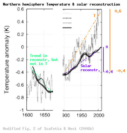
Looking at the SW curves in more detail (their Fig. 2), one of the most pronounced changes in their solar-based temperature predictions is a cooling at the beginning of the record (before 1650), but a corresponding drop is not seen in the temperature curve before 1650. It is of roughly similar magnitude as the increase between 1900 and 1950, but it is not discussed in the paper. As in their earlier papers, the solar-based reconstructions are not in phase with the proxy data. However, SW argue that by using different data for the solar irradiance, the peaks in 1940 (SW claim it is in 1950) and 1960 would be in better agreement. So why not show it then? Why use lesser data?
The curves in Figure 2 (Fig. 2 here shows the essential details of their figure) of the SW paper suggests that their reconstruction increases from -0.4 to 0K between 1900 and 2000, whereas the the proxy data for the temperature from Moberg et al. (2005) changes from -0.4 to more than +0.6K (by rough eye-balling). One statement made both in the abstract of the SW paper and the Discussion and Conclusions (and cited in the senate hearing) is that «the sun might have contributed to approximately 50% of the total global surface since 1900 [Scafetta and West, 2006 – an earlier paper this year])». But the figure in the SW paper would suggest at the most 40%! So why quote another figure? The older Scafetta and West (2006) paper which they cite is discussed here (also published in Geophysical Research Letters), and I’m not convinced that the figures from that paper are correct either.
There are some reasons to think that solar activity may have played some role in the past (at least before 1940), but I must admit, I’m far from convinced by this paper because of the method adopted. It is no coincidende why regression is a more widely used approach, especially in cases where many factors may play a role. The proper way to address this question, I think, would be to identify all the physical relationships, and if possible set up the equation with right dimensions and with all appropriate non-linear terms, and then apply a regression analysis (eg. used in “finger print” methods). Last week, we discussed the importance of a physical model in making attributions because statistical correlations are incapable of distinguishing between forcings with similar trends. Here is an example of a paper that has exactly that problem.
There is also a new paper out on the relationship between galactic cosmic rays and low clouds by Svensmark. We will write a post on this paper shortly.
Tiny point, I’m sure you’ve hit it before.
Peer review is important, so assumptions and data can be questioned. Replication is essential, to see if findings generalize. That’s the difference between micro-critiquing (very popular in some circles) and science, and what really makes this a collective enterprise.
[Response:Hopefully, this kind of exercise motivates authors to take greater care when they design their analytical approach. It’s not a tiny point if the process of peer review starts to slip slide… -rasmus]
If solar is responsible for half of global warming, then all the more reason to reduce our greenhouse gas emissions. We can’t control the sun, but we can alter the greenhouse effect through the amount of fossil fuels we burn.
Re #2: Alastair, if solar has a higher influence than currently implemented in GCM’s, that implies that the effect of 2xCO2 is lower than expected. That means that we have more time to mitigate to non-fossil alternatives… Thus no need to push the panic button, but a huge need for more subsidies for alternative research/implementation.
[Response: No. it doesn’t. CO2 sensitivity is an independent calculation (as I have explained many times). -gavin]
Rasmus,
Much depend of what the historical variability was. If one takes the MBH98/99 reconstruction as base, the variation in the pre-industrial period was ~0.2 K, of which less than 0.1 K (in average) from volcanic eruptions, the rest mostly from solar (I doubt that land use changes had much influence on global temperatures). If one takes the Moberg reconstruction as base, the variation was ~0.8 K, again of which less than 0.1 K from volcanic, thus 0.7 K from solar changes. Or a ratio of 1:7 for solar influence on temperature estimate between the two reconstructions.
As we only have one instrumental temperature trend, the difference between the two estimates for solar sensitivities means that a larger influence must be compensated by a smaller influence of the GHG/aerosol tandem, to fit the temperature trend in the past century…
The pre-industrial historic correlation between temperature and CO2 levels was remarkably stable around 10 ppmv/K, and shows up in the Law Dome ice core as a 10 ppmv change for the MWP-LIA transition. Which points to a change of ~1 K in that period…
As I have said in the other thread, one can easely fit the past century trend with different sets of sensitivities in a simple EBM model (see here, especially by reducing (halving) the sensitivities for GHGs and aerosols in tandem… As the influence of aerosols probably is overestimated (and of solar underestimated) in current GCM’s…
Re 3 (response)
“No. it doesn’t. CO2 sensitivity is an independent calculation (as I have explained many times)” Gavin, do you have a link on this subject ? I still do not correctly understand how the calculation of CO2 sensitivity in past or present climates can be independant from the estimation of the other forcings related to temperature trends (and from natural/chaotic variability). By advance, thanks.
[Response: We’ve discussed climate sensitivity many times (see here) – the specific issue that I think confuses some is that we can’t use the 20th century changes to usefully constrain this because of the uncertainties you allude to. Thus empiricially it must be derived from other sources. Within a model of course, it is absolutely independent. -gavin]
Re #3 and #5
The point to realise is that if the climate sensitivity is 3C for x 2.0 CO2 then the fact that the sun has added a further 0.5C will not make much difference. I think Gavin is arguing that because x 1.3 CO2 produces a much smaller effect, then it will currently be masked by aerosols, the ABC, land use, solar, and the changes in methane levels etc., so we can’t use the current temperature change to estimate the climatate sensitivity of CO2.
I would add that we have already reached or even passed the tipping point, because the melting of the Greenland glaciers is accelerating and they will not stop melting unless the atmosphere cools. So long as we keep increasing atmospheric CO2, then the glaciers will melt faster. One could hope that the sun will get weaker, but that seems highly unlikely if it is indeed causing warming.
If the sun stays the same and CO2 stays the same (we stabilise emissions at today’s level immediately,) then the tempreature will still rise because of climate commitment from the oceans continuing to warm. That means that the Greenland ice is doomed, and the subsequent sea level rise means that Bangladesh, Florida and Flanders are doomed too!
re #6
I agree with you, Alastair, if [deltaT]2xCO2 is 3°C, 0,5°C from solar irradiance variation doesn’t matter. But the problem is precisely the uncertainty of this climate sensitivity, either empirically or theoretically defined. And my question was : in what way can we consider that direct and indirect effects of solar variations on climate (and temperature) are totally independant from this reduction of uncertainty in climate sensitivity.
Thank you for the link, Gavin, raypierre article and comments are particularly interesting.
So, as far I as (try to slowly) understand, XXth century (even the last 1000 years) is unuseful to estimate empirically climate sensitivity because of the too slight variations involved. We must compare more contrasted period, like LGM and PI.
But there’s is still a point on this : when we compare LGW and PI, how are we sure that we include all pertinent factors (others than GHG, albedo of ice, dust and vegetation)? For example, let’s imagine that latitudinal and seasonal variations (Milankovic) of insolation between LGW and PI imply a +/-10% of nebulosity, for some ocean-atmosphere circulation’s reasons. How is it implemented in models ? Or, even more broadly, we know there’s approx. 0,1% variation of solar irradiance between two cycles minima (Willson 2003), how do we exclude with reasonable confidence the hypothesis that there is a 1% variation between 21.000 y BP and 1750 AD ?
Rasmus, do I understand you correctly: Scafetta and West in their paper do the simple analysis by comparing 17th and 18th Century, and by comparing 17th and 19th Century – but they do not discuss the comparison of 18th and 19th Century which would have shown their approach is ill-conditioned? Since this would have taken them a few minutes, given they have all the data for those three centuries, I wonder whether they really didn’t try this before publishing their paper?
[Response:The expression becomes ill-posed when the denominator is zero, which is not exactly what happens for the 19th and 18th century, but these centuries nevertheless illustrate how sensitive the results are. The total solar irradiance (TSI) for 19th century is accoring to SW 1365.64 W/m2, 1364.68 W/m2, or 1365.52 W/m2, depending on whether you use Lean (1995), Lean (2000) or Lean (2005) values. For the 18th century, the corresponding figures are 1365.48, 1364.44, and 1365.43 W/m2. For the temperature anomaly, they use -0.41K for the 19th century and -0.41K the 18th century. Thus for the difference between 18th and 19th centuries, this gives values of 0.50 0.33 0.89Km2/W, depending on which data set you use. I get temperature changes of 1.08 0.54 0.67K respectively (I have put a simple R-script here). -rasmus]
An excerpt related to this paper from an earlier post:
In this paper Scafetta and West reveal an obviously sceptical agenda. They discuss an even higher solar influence, listing well-known and antiquated sceptic’s arguments as the overestimation of 20th century warming due to heat-island effects, or the lower trends in satellite observations. And at last they have found a new one: they suggest that the difference in the temperature increase over land and the oceans during the last decades might be due to contaminations of the land temperature record – They call it an anomalous behaviour – ignoring that it corresponds fully to what is physically expected. Maybe it would help them to have a look at the IPCC report.
The many problems in their analysis have been discussed above and before.
FYI …
Water for Millions at Risk as Glaciers Melt away
by David Adam
October 11, 2006
The Guardian / UK
Excerpt:
Some problems:
1) They appear to have looked at things globally – perhaps looking at regions’ responses would have been better
2) Assuming a direct transfer function between irradiance and temperature, instead of second order effects of irradiance and temperature, or even, instead of other non irradiance measures related to impinging full band EM energy of solar or other extreterrestrial origin, they may have made a bit too much of a leap.
3) They appear not to postulate specifically enough regading mechanisms – for example, postulating a specific role for a specific energy bands’ impingement accentuating or impairing cumuloform cloud formation in the tropics.
It seems unconscionable to me for SW to exclude all contributing factors and claim their results have any merit. In most professional circles I’m familiar with (particularly in aerospace engineering) omitting such obvious factors could bring serious professional consequences. In this field, with lives even more at stake than with those flying an engineered aircraft, it is irresponsible to present such an erroneous result as they did.
RE: #11
SecularAnimist, a good and timely link to the important work of Dr. Kaser and colleagues at the Tropical Glacier Group, Innsbruck University. A link to their publications is
http://tinyurl.com/f9ouh and a further link to that report is:
http://tinyurl.com/lzgrd
Their work builds upon the expanding volume of observed and measured data (including the vital work of Dr. Lonnie Thompson at Ohio State Univ) confirming what reasonable people agree – a warmer world melts glaciers; and perhaps more rapidly than earlier imagined.
RealClimate posted a very informative thread on tropical glacier retreat and is worth a revisit.
http://tinyurl.com/n2lpo
I believe India, Pakistan, Kashmir, Nepal, China will feel the full effect of lost glacier melt runoff that feeds major rivers in their part of the world and provide irrigation and drinking water for tens of millions of people.
Sometimes I wonder if we are all in a collective dream about glacial melt back because it does not appear to be of any real interest to the CIA, National Security Council or the Council on Foreign Relations.
Why am I concerned and they appear to be ignorant of the consequences of losing Himalayan glaciers? Maybe it is simply that I accept AGW and for them to poke into the glacier melt back studies is an admittal there is a looming problem that will dwarf WMD and democratization of the Middle East. Mass migration of hungry and desparate farmers and villages along the norhtern coast of the Indian Ocean is a frightening prospect. Guess the large-brained national security types have their hands full trying to secure our future oil supply. Silly me.
I am surprised that the left hand side of your modified graph is annotated with ‘Trend in reconstr but not in T’
-In the period you’ve shown, if one looks at the low frequency component of the Moberg reconstruction, there is a clear max at around 1630 and a minimum at around 1675.
Smoothing the full Moberg reconstruction yields maxima and minima that are slightly further apart ~1620 and ~1690
The trend over this period is only about a degree which looks to be about a third the size of S&W but they are trends none the less.
Have you cut out the middle of Fig2 so as to stop readers developing unsavoury thoughts, of a solar nature ;-)
speaking of peer review:
I noticed an interesting sounding review entitled “The Global warming Debate: A Review of the State of the Science” in PURE AND APPLIED GEOPHYSICS 162, 1557-1586 (2005). It turned out to be “interesting” but for all the wrong reasons.
I’m a scientist but not a climate scientist (molecular biology actually!). However, it is blatantly obvious that this so-called “review” (by ML Khandekar, TS Murty and P Chittibabu) is a disgraceful and (I would have thought) embarrassing piece of propaganda full of downright falsehoods about the “state of science”.
A number of questions come to mind about this. Clearly the editors of this “journal” (which I assumed was “respectable” but I now wonder) are aware that they have allowed a piece of misrepresentational garbage to appear in their journal. So are they part of, and party to, this process of misrepresentation? In the normal course of events the “scientific process” would pertain. People publishing blatant rubbish would lose their scientific credibility. Authors might think twice before submitting their work to this journal. The paper would be ignored and sink into oblivion. But in “normal” fields of scientific endeavour (like molecular biology for instance) this sort of rubbish just doesn’t happen.
I thought about doing several things, none of which I did in the end. Writing to the editors to express my distaste along with a synopsis of the errors and misrepresentations that are obvious even to a molecular biologist. I considered discussing having the journal subscription cancelled by our university…
Is there a useful way of adressing this problem? Or do we just accept that the normal scientific publication process has been “infiltrated” at several levels (presumably up to the editorial level in this case), and just allow time to deal with the (still very small) misrepresentations and propaganda-dressed-as-science that surprisingly (for me) has been allowed to ooze into the mainstream scientific literature. Or maybe “Pure and Applied Geophysics” isn’t mainstream scientific literature…
this is vey know in my country climate is not very variable
>Mass migration of hungry and desparate farmers and villages along the norhtern coast of the Indian Ocean is a frightening prospect.
If changing to energy intensive agriculture allows more food to be produced by just 2% of Indian farmers on half of the previous land, that should be no more frightening than when the other 98% of US and Canadian farmers migrated to cities in the late 19th and early 20th centuries.
Watching with great interest. Will be back. Barbara
The Kandehar paper was discussed for a while last year, starting here:
http://johnquiggin.com/index.php/archives/2005/07/17/disinterested-sceptics/#comment-29646
Rasmus,
I have purchased (again, AGU must get rich from all those single contributions…) the article. And have some problems with your comment.
– They used the difference between 17th and 18th/19th century as that are the largest differences. Of course, if one uses a smaller difference as like between the 18th and 19th century (about 3:1/4:1), that increases the error margins (the error margin is up to 50% for the 18/19th century difference, 5-20% for the others). But that doesn’t show that the method itself is wrong, or gives unacceptable answers. Thus your Fig.1 end only shows that the error in the scaling factor blows up with smaller differences, which they of course didn’t use to calculate their factors.
– The transfer functions range from 0.20 to 0.57. This is for different solar reconstructions (all by Lean ea.). As the different solar reconstructions only differ in amplitude – not in shape – with the same temperature reconstruction the endresult is (nearly) the same. That doesn’t show any inconsistency in the method used, only that smaller differences in solar reconstruction need larger factors to explain the reconstructed temperature.
– As already said, land use changes probably had (and have) a limited effect on global temperatures, as good as volcanoes (less than 0.1 K). Thus the remaining pre-industrial variability is mostly solar (and internal) variability.
– According to several Antarctic ice cores, there was a ~10 ppmv drop in CO2 between the MWP and LIA, this points to a ~1 K drop in global temperature, which is more in line with the higher variable reconstructions.
– One shouldn’t highlight short discrepancies in the trends, what is of interest is the overall trend.
– The 1900-2000 NH temperature trend is 0.8 K (GISS NH, 5-year smoothed). An extra 0.1 K is added after the year 2000…
Further:
The Moberg reconstruction ends in 1950… thus the comparison for the 1900-2000 period probably uses part of the Moberg reconstruction and part of the instrumental record (for the period 1950-2000). There is a known problem with tree-ring based reconstructions for the period after ~1950, the “divergence problem”, which still is not resolved. Moberg’s reconstruction also uses other proxies, but these are not extended after 1950. This makes any comparison after 1950 (or 1980 for solely tree-ring based proxies) rather problematic.
About the attribution of climate responses to different forcings in current GCM’s, as used in Fig.1 of this page:
– volcanic is overestimated. The Pinatubo (of which strength there were only 9 in the past 600 years, see Fig.6 from Briffa) had an influence of -0.6 K in its peak year, much less in the next years. The decadal average thus is less than 0.1 K. In the beginning of the century there were 2 consecutive eruptions with the same strength (10 years apart). Over the rest of the century, much less. Thus the smoothed variation over the century should be less than what is shown, anyway without positive value (I have never heard of an inverse volcanic effect).
– (sulfate) aerosols are largely overestimated. Because of their very short lifetime (a few days) vs. volcanoes (a few years) for identical physico-chemical reactions, their (primary) effect is less than of volcanoes, despite the higher emission rates (secondary and tertiary effects even are far more uncertain). For a comprehensive overview of all my doubts on aerosol influence, see my comment on RC here.
– But if the (negative) influence of aerosols (and volcanic) is overestimated, the modeled trend would be way too high. That means that the (positive) response to GHGs must be lower than currently implemented in the models (the direct effect – without feedbacks – of anthropogenic GHG forcing is currently ~0.3 K). Thus that 50% of the past century warming may be attributable to solar forcing comes into sight (even in current models with more realistic estimates)…
Last but not least: do you know of trends from any climate model which covers the full 400 year as what S&W did, compared to the Moberg reconstruction, and has that a better performance? I have found Fig.1 in Cubash ea. and a strange graph as Fig.1 in Widmann and Tett (with natural influences-only runs giving higher 1900-2000 temperatures than runs with natural + anthro!). Compare these to the performance of the S&W trends…
>16
The Kandehar paper was discussed for a while last year, starting here:
http://johnquiggin.com/index.php/archives/2005/07/17/disinterested-sceptics/#comment-29646
It’s been cited only once, per Google Scholar, in an article on algae growth on buildings.
Oblivion enough?
I am the author of the paper under accuse, I try to reply to Dr. Rasmus.
(when I finished writing this comment I saw that #21 replied already to Dr. Rasmus, very well, but I add my comments any way. BTW papers may be obtained for free by writing an email to the authors, for example. )
1) The greatest flaw.
Dr. Rasmus uses the differences between averages during the 18th and 19th centuries, while I started from the 17th century, and he found unrealistic results. So Why didn’t I do the same Rasmus’ calculations?
Well, Rasmus adds these comments: “In my physics undergraduate course, we learned that one should stay away from analyses based on the difference between two large but almost equal numbers, especially when their accuracy is not exceptional;” and “hence neglect factors (natural forcings) such as landscape changes (that the North America and Europe underwent large-scale de-forestation);” and “It is, however, possible to select two intervals over which the average total solar irradiance is the same but not so for the temperature. When the difference in the denominator of their equation is small (the changes in the total solar irradiance are small), then the model blows up.”
Well, I think Rasmus has given also answer! It is unsafe to do the calculations comparing the 18th and 19th centuries because the errors will be much larger due to the fact that the averages are very close and because the 19th century would be already partially effected by some anthropogenic factors due to the beginning of the industrialization and some deforestation (that is an anthropogenic component too!!!). So, I used an algorithm that stresses the values during the previous 17th and 18th centuries when anthropogenic contamination is practically zero!!
2) A charm: cutting a picture in two.
By cutting my picture in two, Dr. Rasmus gives the impression that his calculations are fine. The truth is that with my calculation a reader can see an evident correspondence, (that is, a good fit) between the temperature and the solar signal during the pre-industrial (before 1800-1900) era that suggests my results are reasonable. By using Rasmus’ numbers the correspondence would be visibly lost because he gets a double value for the sensitivity that would imply double amplitudes of the reconstructed solar-induced temperature signal that would not fit the data for any of the 4 centuries any more
3) Ambiguities on numbers.
Dr Rasmus writes: “the results gave a wide range of different values for the transfer functions: from 0.20 to 0.57!”
Well Dr. Rasmus did not realize that I am using three different solar records. He should read more carefully my paper. Look at figure 1 !!!
Dr. Rasmus writes: “But the figure in the SW paper would suggest at the most 40%!”
Well, a carefully look would have the solar signal value of -0.45K (1900) and ending at 0.0K (2000), so the difference would be 0.45K. The temperature goes from -0.40K (1900) to 0.50K (2000) (look at the average value between 1950-2000), so the difference is 0.9K. Well, the value is 50%, correct?
4) Galileo, and the inquisition !
Dr. Rasmus writes: “Looking at the SW curves in more detail (their Fig. 2), one of the most pronounced changes in their solar-based temperature predictions is a cooling at the beginning of the record (before 1650), but a corresponding drop is not seen in the temperature curve before 1650.”
Well let us look at the history. Galileo just started to observe the sun-spot since 1611. The sun-spot measurements from 1611 and 1650 are probably quite poor, so the TSI reconstructions during that time are poor because poor are the data. And then there were the religious wars in Europe and the inquisition… I guess that perhaps the 17th centuries guys involved in these matters were to busy to think to fix the measurements to avoid the comments by Dr. Rasmus.
5) A good point.
Dr. Rasmus writes “The proper way to address this question, I think, would be to identify all the physical relationships.”
Well I agree, but today we do not know all the physical relationships, that is why I wrote “To circumvent the lack of knowledge in climate physics, we adopt an alternative approach.. etc, etc…..”
I hope this is helpful.
[Response:Thanks for your repsonse, Dr. Nicola Scafetta. However, I’m still not convinced, as the temperature is not only affected by greenhouse gases and solar activity (take the ice ages, for example…?). I think your choice of method is not robust and is likely to provide wrong answers, and one can illustrate that by applying the same method to the difference between the 19th and 18th centuries (for which you say factors other than solar may play a role – just my point!). You ask me a question: “a carefully look would have the solar signal value of -0.45K (1900) and ending at 0.0K (2000), so the difference would be 0.45K. The temperature goes from -0.40K (1900) to 0.50K (2000) (look at the average value between 1950-2000), so the difference is 0.9K. Well, the value is 50%, correct?” I may misread the figure, but the solar signal seems to be lower than 0.0K at year 2000. An the temperature seems to be greater than 0.50K, but my reading may have been ‘disturbed’ by the fact that not many years later, the temperature exceeds 0.6K. -rasmus]
I’ve been lurking here for years, gathering such understanding as I’m capable of, which is only partial. I just wanted to say how grateful I am and admiring of your efforts, integrity, and dedication. Your science is beautiful and crucial. We need you guys.
Perhaps Steve Reynolds (#18) missed the stories in the NY Times regarding groundwater depletion and problems with surface water supplies in India. Or he has never heard of the fate of the agricultural production dpendent on the Ogalala Aquifer?
The URL for the reconstruction of volcanic influences from Briffa ea. can be found at:
http://www.cru.uea.ac.uk/cru/posters/2000-03-TO-mendoza.pdf (Fig. 6).
It looks like that current models simply have adopted the Briffa reconstruction (compare Fig.6 of Briffa with Fig.1 on this page), without looking at the physical evidence…
Re 23
Dear Nicola
Sorry, but your explanations did not help very much yet. There remain several questions, e.g.
– You state that Sun spot observations before 1650 are poor. However, this is half of the data for the 17th century value. This would mean, your value for the 17th century is poor and in fact you shouldn’t use it.
– You state that the measurements in the 19th century are already anthropogenically influenced. This means that your value in the 19th century has an anthropogenic influence and is not only solar induced.
– According to your Zs values, the error bars and the TSI values, the temperature should have increased from the 18th to the 19th century between 0.03 and at most 0.06. In fact, the increase was 0.08, which is between 30 and 160% more. You seem to explain this by possible anthropogenic influence. However, if the anthropogenic influence in the 19th century possibly is more than 50%, how can you use the value of the 19th century in a calculation which assumes nearly 100% solar influence?
Thus, if the data is poor before 1650 and is possibly anthropogenically influenced after 1850 it might be more appropriate to compare 1650-1750 and 1750-1850.
A rough estimate from the graphs shows that you would get Zs values between about 0.10 (or even below) and about 0.25 for the three TSI reconstructions, which is about half of what you get.
And a last question:
You compare different TSI reconstructions. Why don’t you also compare different temperature reconstructions?
[Response:I think that the sunspot data for the 18th and 19th is questionable as well, because there are something strange happening to solar cycle length. -rasmus]
Rasmus, I cannot convince everybody!!!
You write: “that by applying the same method to the difference between the 19th and 18th centuries (for which you say factors other than solar may play a role – just my point!).”
Yes, Rasmus, by doing the calculations as you want to do them, the result would be not robust. That is why I chose to do the calculations in a different way.
You are criticizing your own calculations and your own methodology, not mine!!!
About the numbers in the paper I wrote “approximately 50%”, the error is about 15-20% of that value. So, it is fine.
A short reply to #27
1) I use the reconstructions that are available. All reconstructions might have problems.
2)I did not use the 19th century at 100% value but an agorithm that stesses the 17th and 18th century values, and then I checked that the things look OK.
3) In the paper I used Moberg data because these data are the latest one. And because in GRL we have a limited number of pages.
[Response: Rasmus’ point is I think more general. In any period there will likely be more than one thing going on. This is as true for the 17th Century as for the 19th Century. These ‘other things’ (principally volcanoes, but also land use etc.) are presumably uncorrelated with solar forcing over the long term, but in the absence of enough centennial cycles in the observational record, one can’t assume that you can average over them by taking enough examples. In the late 17th Century for instance, our work has suggested about a 50-50 split between volcanic and solar effects (compared to the late 18th Century) which enhances the global cooling. Other studies have come up with other splits – including some which find a dominant role for volcanic forcing. It’s not easy to distinguish between the two (given the uncertainties in the forcing data), but it might preclude one from simply assuming that it was all solar. -gavin]
[Response:I think we are not quite on the same frequency (to give you a clue – I’m not critising myself, but only demonstrating that you method is not reliable), and I hope that Gavin’s explanation helps. On a more specific issue, even counting in errorbars, the usual way to do this is this to center the range around the best estimate, so you should have written 40% +- error. How did you estimate the error, is it one standard deviation or the 2.5-97.5 quantiles? (by giving a range 15-20% gives me the impression of being a bit handwavy, but 20% of 40 is 8, right? And that upper limit is not the most likly estimate…) But the figure is reproduced above, and the readers can make up their own minds. -rasmus]
Study Links Extinction Cycles to Changes in Earth’s Orbit and Tilt
By JOHN NOBLE WILFORD
If rodents in Spain are any guide, periodic changes in Earth’s orbit may account for the apparent regularity with which new species of mammals emerge and then go extinct, scientists are reporting today.
It so happens, the paleontologists say, that variations in the course Earth travels around the Sun and in the tilt of its axis are associated with episodes of global cooling. Their new research on the fossil record shows that the cyclical pattern of these phenomena corresponds to species turnover in rodents and probably other mammal groups as well.
In a report appearing today in the journal Nature, Dutch and Spanish scientists led by Jan A. van Dam of Utrecht University in the Netherlands say the “astronomical hypothesis for species turnover provides a crucial missing piece in the puzzle of mammal species- and genus-level evolution.”
In addition, the researchers write, the hypothesis “offers a plausible explanation for the characteristic duration of more or less 2.5 million years of the mean species life span in mammals.”
Dr. van Dam and his colleagues studied the fossil record of rats, mice and other rodents over the last 22 million years in central Spain. The fossils are numerous and show a largely uninterrupted record of the rise and fall of individual species. Other scientists say rodents, thanks to their large numbers, are commonly used in studies of such evolutionary transitions.
As the scientists pored over some 80,000 isolated molars, the most distinct markers of different species, the patterns of turnovers emerged. They seemed often to occur in clusters, which seemed unrelated to biology. And they occurred in cycles of about 2.5 million and 1 million years.
continues in link…..
http://www.nytimes.com/2006/10/12/science/earth/12extinct.html?ei=5065&en=83d5e73f9f09c803&ex=1161316800&partner=MYWAY&pagewanted=print
I think they learned it from watching so called climate scientists do the same thing when they focus all the “blame” on CO2.
[Response: Why not try reading what we ‘so-called’ climate scientists actually say?
Sorry to be snippy, but it can get a little tiresome to always be dealing with strawmen arguments…. – gavin]
In the 20 or so AOGCM models used by IPCC, for simulation of XXth and projection on XXIth centuries, do you know how many use some varying value for solar radiative forcing and how many consider it as constant (or ignore it as insignificant) ?
[Response: In the 19 models studied in Santer et al (2005) (Table 1), 11 models have historical variations in solar irradiance, 7 don’t, and one was uncertain. I’m sure there is a better description of the specific forcings for each model somewhere, but I don’t know where (anyone?). – gavin]
It seems to me if you only can get the given result by using a particular pair of 100 year intervals you are in deep doo doo. For example, if you start using 1600 to 1700, how does the result change if you use 1610-1710, 1620-1720, etc. As Gavin points out, what is being done is to pick one particular set of differences from a set of measurements which are both noisy and not particularly well known.
Also wrt #18, the Enclosure Acts did not lead to a life of milk and honey for the displaced farmers and in the US, for example, the life of the Okies displaced from their farms by an ecological disaster was not celebrated for the ease and luxury they found in the cities.
Re #29: We are a bit off topic here, but I saw this article and would like to know which 2.5 million and 1 million orbital cycles they are talking about? The eccentricity and obliquity (axial tilt) cycles they mention have periods of about 100,000 and 22,000 years respectively.
Regarding #16 and #22,
It’s always interesting to read a paper like the one you reference and then take a look at who the authors are and what their background is.
Here’s a quote from the paper: “”During the long geological history of the earth, there was no correlation between global temperature and atmospheric CO2 levels. Earth has been warming and cooling at highly irregular intervals and the amplitudes of temperature change were also irregular. The warming of about 0.3 C in recent years has prompted suggestions about anthropogenic influence on the earthâ��s climate due to increasing human activity worldwide. However, a close examination of the earthâ��s temperature change suggests that the recent warming may be primarily due to urbanization and land-use change impact and not due to increased levels of CO2 and other greenhouse gases.” This is a nonsensical view.
Khandehar has previous record on this issue; for example at http://gmopundit.blogspot.com/2006/09/indias-successful-agricultural.html :
“INDIA’S ECONOMIC PROGRESS IN A CHANGING CLIMATE: BENEFITS OF GLOBAL WARMING
As a weather & climate scientist, what impressed me was the fact that India’s strong economic progress has come about in an increasingly warmer world of the last forty years or so, completely defying the projections of deleterious impact of Global Warming by IPCC (Intergovernmental Panel for Climate Change, a United Nations Group of Scientists) and its supporters.”
What about the other authors? Tad Mundy has published a fair number of papers on tsunamis, but nothing on climate – last time I checked there was no relation between earthquakes and global warming. This paper is his first on climate change – generally ‘reviews’ are written by leaders in their field. P Chittibabu has published a few papers with Tad Mundy on tsunamis, but that’s it. Of more interest is his employment with W.F. Baird and Associates, a coastal engineering firm that also sells 3D imaging software – a little research into this firm reveals that one of their main clients is likely the Canadian petroleum industry. It’s highly likely that restrictions on Canadian CO2 emissions would hurt their bottom line. See http://www.esricanada.com/english/solutions/wfbaird.asp and also http://www.esricanada.com/english/nresources/default.asp#petroleum for more.
As #22 points out, this paper has been ignored by the climate science community. That’s not the problem – the paper is available at http://www.friendsofscience.org/documents/debate.pdf . Who is “friends of science?” Here is the lead statement from their website: “The Kyoto Protocol is a political solution to a non-existent problem without scientific justification”. This paper is used to promote that notion outside of climate science circles.
So why go to all this trouble? In a nutshell – Canadian tar sands in Alberta. See http://www.ualberta.ca/~parkland/research/perspectives/GassyElephant06OpEd.htm – as they point out, “The tar sands are the single largest contributor to the growth of greenhouse-gas emissions in Canada, because it takes so much of Canada’s diminishing supply of natural gas to make tar sands oil. Greenhouse-gas intensity in the tar sands is almost triple that of conventional oil. As Jim Dinning, Alberta’s former treasurer and front-runner to replace Ralph Klein as Alberta’s premier, recently quipped, “Injecting natural gas into the oil sands to produce oil is like turning gold into lead.”
This really represents a serious abuse of the scientific process, and the journal’s editors should know better. Is it appropriate to email the journal editor and ask what happened to the review process? Well – that’s what I did, so we’ll see.
I imagine that these papers on solar influence on climate will also be widely posted on sites like ‘friends of science’.
Re #33. The 100,000 and 22,000 year cycles coincide periodically. Technically they should coincide every 1,100,000 years (the least common multiple of 100,000 and 22,000) – but the cycles are not exactly 100,000 and 22,000 – and the time actually varies slightly depending on extraterrestial forces (the other planets) and internal Earth dynamics (position of tectonic plates, cryosphere, core flows?). So the cycles theoretically are estimated to coincide at the times specified in the past [those calcuations have inherent approximations due to limitations of underlying estimates required to make them].
Rodent extinctions in Spain correlating with this cycle is quite interesting – but obviously hardly decisive evidence. The crux of the hypothesis being that mammals would have a survival advantage over (reptiles?) during periods of high seasonality and vice-versa during periods of low seasonality – primarily I suppose due to food mix changes, temperatures and disease carrying insects.
A cousin of mine who is a Physicist and worked in solid state manufacturing, is a total climate change denier, he reasons that Carbon dioxide has insignificant interaction with infrared radiation (as compared with H2O), therefore the increased levels of Carbon dioxide cannot be influencing climate.
I believe that it is the case that Carbon dioxide has little interaction with the higher frequencies of infrared, however, I suspect that it is the lower frequencies of infrared that interact more with Carbon dioxide.
I have tried a Google on the issue and end up with too many hits that all seem to be about unrelated issues.
Can anyone please tell me the details for infrared – Carbon dioxide interactions, or direct me to a reference in which it is described? I doubt that anything would change my cousins mind, however I would like to give others (to whom my cousin has preached) the details in order to put them straight on the issue of whether or not Carbon dioxide is a ‘greenhouse’ gas.
Cheers,
Lawrence.
[Response: You could try: https://www.realclimate.org/index.php/archives/2005/04/water-vapour-feedback-or-forcing/ or https://www.realclimate.org/index.php/archives/2006/01/calculating-the-greenhouse-effect/ but maybe something more technical is called for… – gavin]
Re #36
Thank you Gavin, however, it is not the actual detail I require. I am actually looking for the infrared properties of CO2, that is the frequencies that it absorbes and the frequencies that it is transparent to. Perhaps emmisivity properties of CO2 may be important as well. Can anyone help?
Cheers,
Lawrence
Re 28,32
That is exactly the point. The results of SW (the Zs values) for a specific TSI reconstruction vary by a factor of about 4 to 5 (e.g. at least between 0.10 and 0.50 for the Lean 1995 reconstruction) depending on the pair of 100y intervals out of the 1600 to 1900 period you chose. With the SW method in that paper you can get almost any result you want – just by chosing the intervals. The reasons for that were well explained by Gavin.
I’m still waiting for a comment of Nicola Scafetta on that point.
Re #36 Lawrence, your cousin is correct that the greenhouse effect of water vapour, and even more so clouds are much larger (x 2 – x 4) than that from CO2. However, the greenhouse effect from water vapour is due to a (positive) feedback from the temperature and so any warming caused by CO2 is amplified by water vapour. In other words increasing CO2 has three to four times the effect one gets by just calculating the changes due to its radiative effects.
A second point to note, which I do not recall having seen elsewhere, is that CO2 has more effect in cold regions than in hot. In other words, in cold regions where the ground is covered by ice or snow, then the vapour pressure of water vapour is low, and CO2 is the dominant greenhouse gas. In the tropics, where the humidity is high, then the effect from CO2 is very much less significant.
This means that while the effect of an increase in CO2 on global temperatures is small, it does cause the snow line to rise in altitude and latitude. This reduces global albedo, and consequently the additional heat absorbed from the sun acts as another positive feedback raising global tempreatures. But, more importantly, it doss not alter the temperature uniformly over the globe. There is a polar amplification which will disrupt the current climate system, and create havoc with agriculture which is now finely tuned to the current climate. Chaos in agriculture inevitably leads to famine.
Re #36: Short answer – the error your friend is making is to look at the relative concentration of water vapor and carbon dioxide near the Earth’s surface. Most of the greenhouse effect takes place in the upper atmosphere where water vapor levels are relatively much lower. The issue of which infrared bands are absorbed is not very relevant.
RE #34: Off Topic, oil sands:
Sometime in the 90’s I read an article in scientific american that predicted “minning oil sand would become economically feasible by the year 2010”, the reason was dimminishing oil supplies and increased consumption (ie: peak oil and all it’s associated mayhem).
Another thing I have seen predicted is that climate change and mono culture could bring about a global food crisis. Here in Australia our (grain) crop estimates have been cut in half (it’s dryer and rains at the wrong times) and our last bannana crop was wiped off the map by a cyclone. My own morbid prediction is we will see farmers bulldozing piles of dead sheep around jan – febuary.
I belive (but am not sure) that the mid west also has similar but less severe problems, and Europe has suffered a “mixed blessing”. I would like to think that I am wrong and we will “somehow” avoid a sudden and painfull population “implosion” within the next generation or two. Fiffty years of experince assisting humanity to screw up, and a high school experiment with fast breeding bugs, tells me otherwise. :(
The Milankovitch cycles are not the same every 100,000, 41,000 and 22,000 years but oscillate around cycles of millions of years where by at some points dueing these cycles (1 in 20 say) the cycle is very bad for warmth and good for Ice and Snow. All Milankovitch cycles are not created equal.
Lawrence, look at the first link in the sidebar under Science
http://www.aip.org/history/climate/index.html
You could get your cousin the book and refer to the website, which is an extended version of the book. Having been a solid state physicist he will probably understand it from there.
Re #28 Gavin’s comment:
Gavin,
Your calculation of the relative impact of volcanic vs. solar is based on the MBH99 (and earlier) proxy variability in the pre-industrial period, which are the proxies with the lowest variability. If more recent proxies are used (Esper, Moberg, bore hole reconstructions), the influence of volcanic in the total variability reduces to ~14%, instead of 50%.
[Response: No. The split was from the individual GCM experiments using best guess forcings. – gavin]
Further, the (every 12 year) repeated simulation of the Pinatubo eruption in Shindell, Schmidt, Miller and Mann gives a value of -0.35 K over the full period. The observed values are -0.3 K for the first and second year after the eruption and essentially zero in the third year. Thus the 12 year average global cooling for this type of eruption is 0.05 K. Maybe I have underestimated the long-time effects of repeated series, but the difference between observed and simulation seems much too large to me…
[Response: There is a cumulative effect which explains the difference, but with a mixed layer ocean I wouldn’t stand by that exact number. The issue we were really looking for was whether there was a different spatial signature in the volcanic-induced cooling which could be used to distinguish it from solar cooling – and there was: volcanic long term cooling was much more homogenous than solar-induced cooling. That remains, I think, the best hope of trying to distinguish the two effects. – gavin]
Re 38
dear Urs Neu,
In physics the calculations are not done by blindly appling a methodology to a set of data. This is what computers do, not humans, who are supposed to be smart!
One should think first, and think for sufficient long time to exploring a lot of different options.
One first has to look at the data, second has to decide what is the most reasonable way to do the calculations and finally has to compares the results with the data to see if everything looks good. If something goes wrong, he has to start again and think deeply.
My choice was made in such a way to yield to a low relative error and a good correspondence between the curves during the pre-industrial era. Rasmus’ calculation, on the contrary, yield to the highest relative error (double than mine) and would produce the worst data correspondence. Moreover the 19th century is already a little bit contamineted, so it should not be used at 100%.
That is why Rasmus’ way to apply my methodology is scientifically unwise and incorrect.
By looking at my full picture, instead of cutting it in two as Rasmus did, you would realize that by using Rasmus calculations the good correspondence seen in the data would be complitely lost for all 4 centuries.
I hope that this help.
[Response:Sorry, but no Nicola. You say that you look at the data and then choose the method. And, besides, what information do you really have about the data and their quality, if you do not take into account other facors? (how can you judge the data, when you forget that factors other than GHG and solar may play a role?) how do you justify using Moberg et al’s temperature reconstruction, and not the others? I demonstrated that your method is unsuitable. I think you do it the wrong way round: first you need to design a method that will give you a objective answer and that is not unduely influenced by noise or external factors, and then apply this to your data. This is the reason why your method is – as far as I know – never used in e.g. the statistics community. -rasmus]
Urs,
The 50% +/- 20% which is found by the method which S&W used is not that different of what Stott ea. found with their optimal detection HadCM3 experiments, where they increased solar and volcanic with a factor 10 and 5 resp. The best estimates for the 1900-1950 period were 40% solar (Lean ea. 1995) and 60% for the Hoyt & Schatten (1993) solar reconstruction. This reduces to 16% and 36% resp. for the two solar reconstructions in the 1950-2000 period.
These findings are within the constraints of the HadCM3 model, where they didn’t vary the influence of aerosols. With a lower influence of aerosols, optimal detection might be more towards solar…
http://adsabs.harvard.edu/abs/2005JCli…18.4824H
Just thought I would add this reference.
At some point, the “warmers” will have to confront the reality that, even if they are correct in general, not every study or fact will support their argument, OK?
So, if someone publishes something that does not support AGW, it’s OK. You don’t have to immediately look for any weakness in the study and heap scorn on the the authors and their methods.
That’s what the skeptics do.
[Response: You make a fair point, which is already accepted. We’re not attacking the study for its conclusions, but for weaknesses in its methods – William]
Re #47:
To be fair to the RealClimate moderators, they also post critiques of articles in the literature which would tend to increase concern about climate change. An example would be concerns about a shutdown of the thermohaline circulation. Again, the argument isn’t with the conclusion, but with the scientific arguments leading to it.
Just by the way … it has an interesting ring to it but I don’t think the first word in the title of the paper is “phenomomenonological”.
[Response: Thanks. I changed it above. You know how it is with these long words… who has the energy to get to the end? ;) – gavin]
Re 45
Dear Nicola Scafetta
Thank you for teaching me how physicists work.
Unfortunately this general explanations do not answer my questions. Your comment is once more on the article of Rasmus but not on my questions. Maybe I can specify according to your response:
1. Does the comparison of the periods 1650-1750 and 1750-1850 result in a higher relative error than 1600-1700 to 1700-1800 or 1600-1700 to 1800-1900, respectively?
How much is the difference between the relative errors?
2. If the difference of the relative errors is similar, wouldn’t it be better to avoid the periods 1600-1650 with poor data and the end of the 19th century which is contaminated? Wouldn’t it be smart thinking to avoid bad data, if better data is available?
3. How do you explain, that choosing 1650-1750 and 1750-1850 instead of 1600-1700 and 1700-1800 gives such a different result?
And another question arising from your answer:
Did you really choose your data periods in a way that there was the best fit of your calculated curves to the temperature curve? Do I get that right?